Features
HIPAVE (Heavy Industrial PAVEment design) is for the mechanistic analysis and design of flexible pavements subjected to the extremely heavy wheel loads associated with freight handling vehicles in industrial facilities, in particular, intermodal container terminals. It is designed to conveniently model each combination of vehicle model and container load and to combine the damage using the Cumulative Damage Factor concept.
Vehicle Loadings and Traffic in Detail
HIPAVE lets you define your vehicle loadings and traffic in detail.
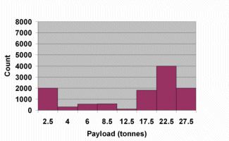
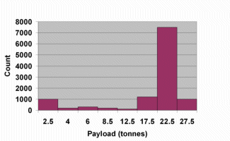
You define the anticipated repetitions over the design period for each vehicle model. You also define a payload distribution for each vehicle model.
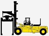
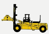
The following example illustrates the concepts. Here there are two vehicle models, A and B. Each vehicle model is assigned a payload distribution.
Vehicle Model A
Vehicle Model A – Payload Distribution
Vehicle Model B
Vehicle Model B – Payload Distribution
Full Spectral Analysis
HIPAVE accumulates the contribution from each loading in the traffic spectrum at each analysis point by using Miner’s hypothesis.
The procedure takes account of:
- the design repetitions of each vehicle model/payload combination; and
- the material performance properties used in the design model.
This approach allows analyses to be conducted by directly using a mix of vehicle models. It is not necessary to approximate passes of different vehicles or axles to passes of an “equivalent” standard load or “design vehicle”.
HIPAVE does a full spectral analysis of pavement damage by using the cumulative damage concept to sum the damage from multiple vehicle models and payload cases for one set of layered system material properties. The figure below is a sample cumulative damage plot produced by HIPAVE:
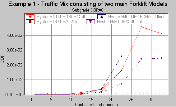
Note that there is a data point for each combination of vehicle model and payload.
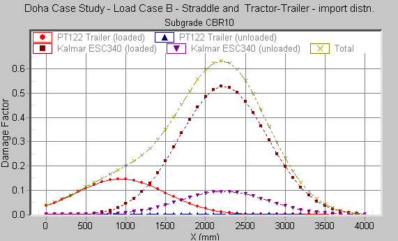
HIPAVE can also generate graphs that show the variation of the damage factor across the pavement, as shown below:
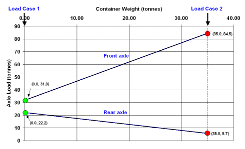
For vehicles that typically have unequal loads on each axle, the vehicle loading characteristics are specified in terms of two load cases that express the axle loads as a function of Container Weight. For example this could be the Unladen case together with one specific Container Weight.
The graph below illustrates the concept. Axle loads for other container weights are obtained by linear interpolation.
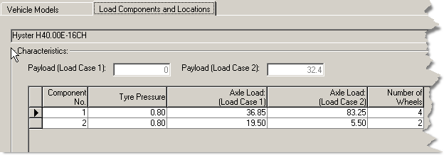
These screendumps show some sample data:

Container Weight Distributions
HIPAVE lets you specify detailed container weight distributions. For example, the British Ports Association Guide (3rd edition) includes frequency data based on data provided by UK ports. The following graph shows the container weight distribution for 40 foot containers.
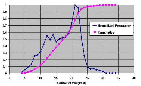 British Ports Association (1996) – 40 ft containers
The container weight distributions are categorized as being “Standard” or “Custom”. The “Standard” distribution feature lets you re-use a particular distribution across a range of vehicle models and projects. The “Custom” distribution is used for just one traffic spectrum / vehicle model combination.
Dynamic Load Factors
So-called Dynamic Load Factors were introduced in the British Ports Association Design Guide (British Ports Association, 1988) to account for the effects of dynamic loading induced by cornering, accelerating, braking and surface uneveness. These are simple multipliers that are applied to the design loads and can vary with each axle. HIPAVE lets you use your own values for the factors.
Cost Optimization
A Parametric Analysis feature can loop through a range of thicknesses for one or two layers, while simultaneously designing the thickness of another layer. This feature will optimise up to three layers. Combining this with a Cost Analysis feature, allows for fine-tuning of layer thicknesses to minimize construction and maintenance costs.
For example, for the pavement structure shown below, you can automatically determine the thicknesses of the Base and Subbase that will minimize the total cost.
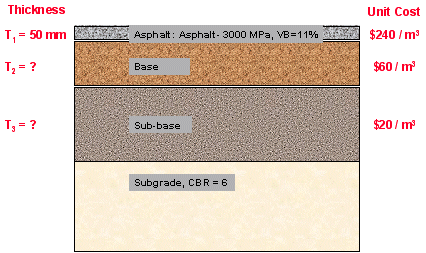
This automatically generated graph shows you the pavement configuration that corresponds to minimum total cost:
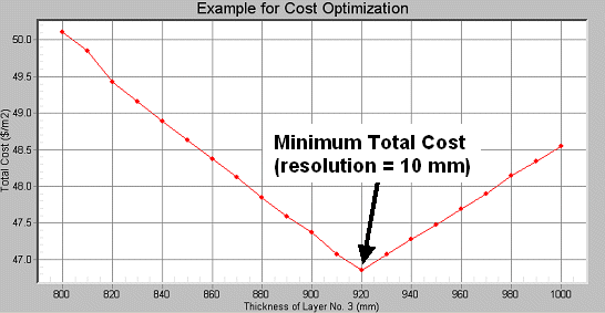
Automatically generated plot: Total Cost vs. Layer 3 Thickness
Click here for recorded Demonstrations.
download the Product Brochure:HIPAVE Overview
System Requirements
- Microsoft® Mouse or compatible mouse.
- Microsoft® Windows Windows 7, Windows 8.x , Windows 10 or Windows 11.
(Compatible with both 32-bit and 64-bit versions.)


